Cloud Resilience

Resilience beyond the obvious #2: Hedging pattern and tail latency

August 03, 2026

TLDR: The hedging pattern boosts resilience by using speculative redundancy to reduce an application’s exposure to tail latency. That’s a rather pompous-sounding phrase, isn’t it? But the idea is simple: launch a primary request attempt to a destination, wait for a duration based on the operation’s expected behavior, and—if it takes longer than that threshold—send a second attempt via another plausibly healthy path. The application uses the first valid response and cancels the losing attempt (or limits its cost). Today’s topic is the hedging pattern and tail latency; I’ll mention upfront that we’ll see plenty of numbers in this article, along with a bit of math (hopefully correct).

In distributed systems, not every failure appears as unavailability. Often a dependency keeps responding, but responds too late: a replica goes through a GC pause, a local queue grows, a network route gets worse, a specific partition becomes temporarily slower. The hedging pattern increases resilience when it prevents that localized variation from defining the application’s final experience.

The pattern only works well when there is independence between paths, idempotency, cancellation and a budget for extra load. Without these controls, the same mechanism that should mask a localized slowdown can double traffic during a correlated degradation and turn protection into incident amplification.

From constant work to the hedging pattern

The first article in this series discussed the constant work principle: avoid making the system execute a different, less exercised or heavier path exactly during a failure. The central idea was to reduce operational surprise. A resilient system needs to behave predictably when a dependency degrades.

The hedging pattern uses a different technique, but seeks the same result: predictability. Instead of keeping the amount of work always the same, it allows a small amount of redundant work to reduce exposure to the worst replica, worst path or worst queue at that moment.

The essential difference is control. Hedging is not duplicating everything. It is not always sending two requests. It is not trying to compensate for lack of capacity with more load. The pattern only makes sense when redundancy is speculative, idempotent, sent to another plausibly healthy path and limited by a budget.

How the hedging pattern increases resilience

The short answer: hedging increases resilience when it prevents a transient and localized slowdown from becoming the user’s experience. It does not make the backend faster by itself, it does not increase real capacity and it does not fix saturation. What it does is different: it reduces the application’s dependence on the slowest participant in a distributed composition.

Think about a checkout flow that needs to fetch risk, balance and history data before responding. All dependencies are available. Nothing is down. But one replica of the history service entered a GC pause, or got a bad local queue, or got stuck behind a temporarily worse network path. Without hedging, the entire checkout inherits that bad luck: the user waits for the slow replica. With hedging, after the p95 the application tries another path and uses the first valid response. The hiccup still exists inside the system, but it no longer crosses the boundary to the user.

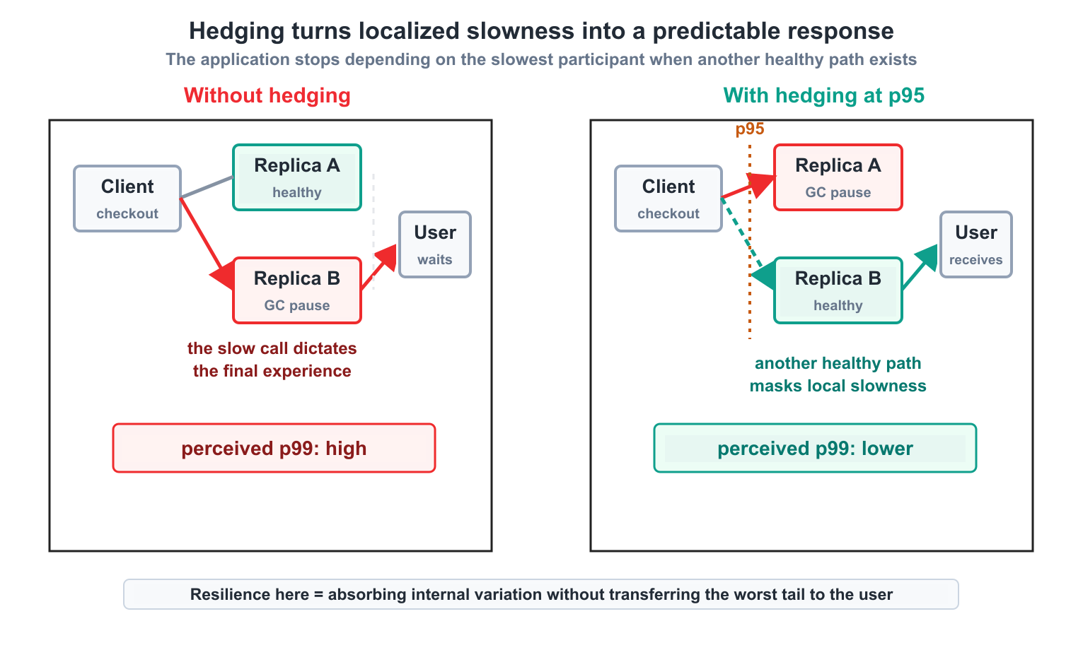
Hedging does not replace redundancy. It uses existing redundancy selectively to absorb internal variation. Without a hedge, a slow replica can decide the perceived latency; with a hedge, another healthy replica can respond before the slow request defines the experience.

This is where the pattern belongs in a resilience conversation, not only in a performance conversation. Resilience is not only continuing to be available when something fails completely. In distributed systems, many things do not go down: they become slow, partial, intermittent or asymmetric. Hedging operates in this range of degradation. It turns a problem that would be visible to the user into a masked internal variation.

A small Python model shows the mechanics without any library:

def without_hedging(primary_ms):
    return primary_ms

def with_hedging(primary_ms, backup_ms, hedge_after_ms):
    if primary_ms <= hedge_after_ms:
        return primary_ms

    return min(primary_ms, hedge_after_ms + backup_ms)

history_primary = 180  # replica with a GC pause
history_backup = 24    # another healthy path
hedge_after = 30       # expected p95 for this call

print(without_hedging(history_primary))                 # 180 ms
print(with_hedging(history_primary, history_backup, hedge_after))  # 54 ms

The second number is not 24 ms, because the hedge does not fire at time zero. The application waits 30 ms before deciding that the first attempt entered the tail, so it pays 30 + 24 = 54 ms. This is the correct design: the system does not duplicate work for all traffic; it buys an escape route only when the original attempt has already crossed the expected threshold.

Also notice what this example does not promise. If the entire history service is saturated, or if both replicas hit the same hot partition, the backup does not return in 24 ms; it returns slowly too. In that case, hedging does not absorb variation, it amplifies load. That is why the pattern only increases resilience when three things are true at the same time: there is another path with a real chance of being healthy, the operation tolerates duplication, and the extra load has a ceiling. Outside that boundary, it stops being protection and starts making the incident worse.

What is the hedging pattern

The name comes from finance: a hedge is a protective bet, something you do in parallel to cover the risk of the main bet. Applied to requests, the concept is: instead of sending the request to one replica and depending on it being fast, send it to more than one and use the first response that arrives. With Dean and Barroso’s paper, The Tail at Scale, the idea they called hedging became popular: send the same request to multiple places and use the first one to respond. It is not quite that simple, and I recommend reading the paper.

If this is done naively, firing two requests every time, for all traffic, you have just doubled your system’s load. Every request became two. This is expensive and, as we will see in the analysis of incident amplification, it can be catastrophic. The important point in the paper is not merely the idea of executing on multiple replicas. It is the refinement that makes the idea cheap: you do not fire the other request, the backup, immediately. You send the first request and only fire the second after a small delay, and you cancel the pending ones as soon as the first good response arrives.

A common starting point for the firing delay is the p95. You delay the secondary request until the first one has already crossed the expected p95 for that request class. The logic is direct: if the first request responds before the p95, you do not send the second and you do not add load. Only when the first attempt enters the tail does the hedge fire. By definition, this limits extra load to approximately 5% while shortening the tail. The cost of redundant work is paid where it actually reduces exposure to tail latency.

The diagram below shows the complete flow. Notice the exact moment when the client decides to fire the hedge: not at the beginning, but after waiting until the p95, and then canceling the slow replica as soon as the fast one responds.

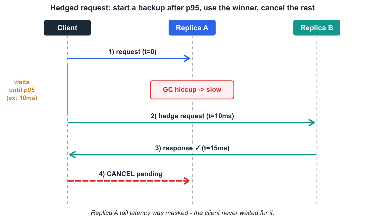
One implementation trap is this: the hedge only helps if it reaches somewhere else. This does not happen automatically. If the second request uses the same hostname, the same key and the same HTTP client, it can land on the same slow backend. The most common causes are keep-alive connection pools reusing the already-open connection; consistent hashing routing the same key to the same node; and sticky sessions in the load balancer. The practical rule is to explicitly force a new connection or a different replica from the first one. A hedge that lands in the same place is not protection; it is additional load on the same bottleneck.

The most cited result from the paper shows the magnitude of this effect. In a benchmark that reads 1,000 keys distributed across 100 storage servers, sending a hedge after only 10 ms of delay reduced p99.9 latency from 1,800 ms to 74 ms, with only 2% extra requests. A 96% tail reduction for 2% more work. That is a trade-off large enough to deserve architectural attention.

If you want to see the effect across the whole distribution instead of one percentile, the distribution explains better why this does not mean the entire system became faster, and it refutes the idea that hedging “makes the system faster”:

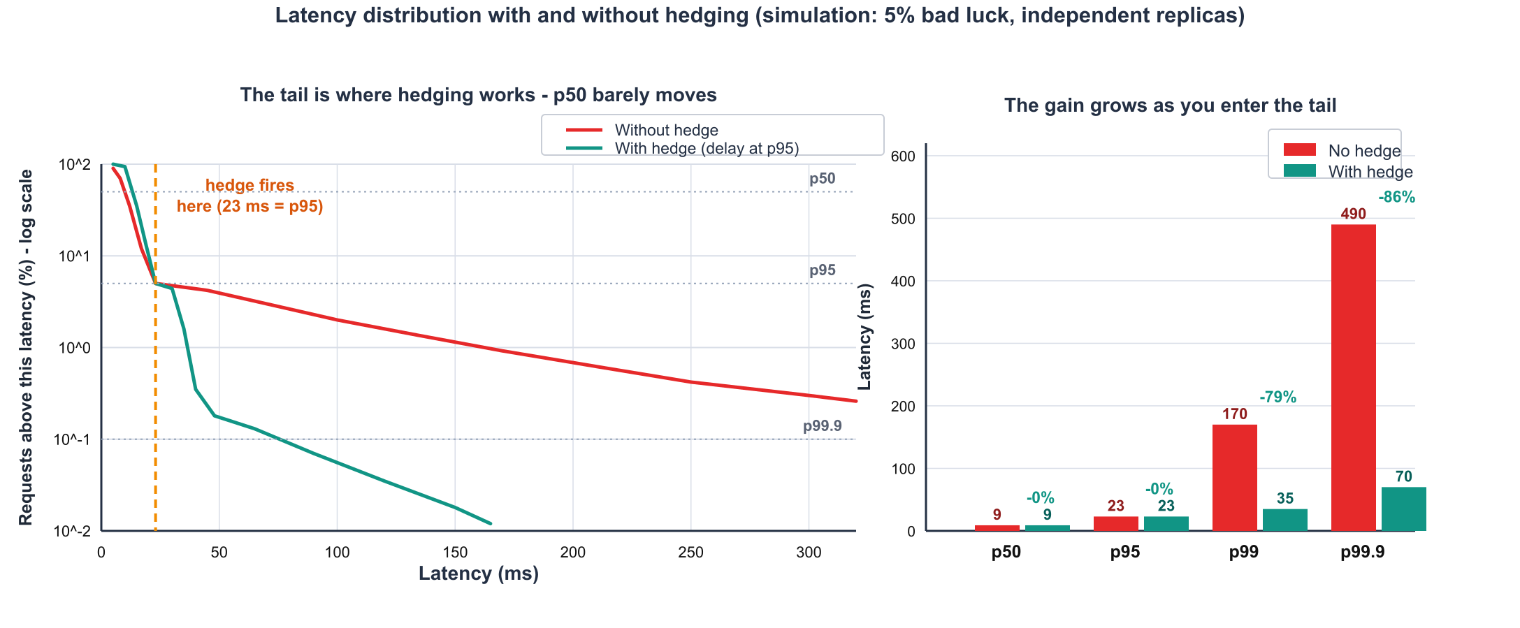
Simulation with 5% bad luck and independent replicas. On the left, the fraction of requests above each latency value, on a log scale: the two curves are identical until the p95 and diverge only in the tail. The hedge does not touch p50 (9 ms to 9 ms) or p95 (23 ms to 23 ms); it reduces p99 (170 ms to 35 ms) and p99.9 (490 ms to 70 ms). Hedging does not accelerate the body of the distribution. It reduces the tail, at a cost of about 5% extra requests.

The mechanism behind this disproportionate gain is tail math working in the application’s favor, with one central condition: the two slowdowns need to be independent. Under independence, the math is favorable: if each replica has a 1% chance of being slow, both being slow at the same time has a 0.01% chance, one in ten thousand. The probability of simultaneous bad luck was squared. But the important word is independent: it returns in the applicability analysis, because it is the most fragile assumption in the whole article.

Hedging, retry, failover and constant work

Hedging becomes clearer when compared with retry, failover and constant work. The four techniques deal with degradation, but each one has a different trigger, scope and risk.

	Hedging	Retry	Failover	Constant work
When it fires	After p95, with the original still in flight	After failure or timeout	Replica/region declared unavailable	Never “fires”: always runs the same
Posture	Proactive	Reactive	Reactive	Neither one nor the other
What it solves	Localized latency tail	Transient and isolated failure	Availability	Predictability under failure
How it fails badly	Doubles load under correlated latency (metastable failure)	Retry storm	Secondary without capacity	Waste in normal operation
Mandatory brake	Token bucket + cancellation + deadline	Backoff + jitter + attempt ceiling	Reserved and tested capacity at target	-

The most important distinction is the proactive-reactive axis. Retry is reactive: it waits for the request to fail, through an error or timeout, and then sends it again. Hedging is proactive: it does not wait for failure, it reacts to slowness, firing a backup while the original is still alive and might still respond. If your problem is requests that will complete, but ten times slower because of transient bad luck, retry is the wrong tool: you would wait for the thing to fail, which may never happen, and by resending you would add load to a backend already under pressure. If your problem is a real failure, the replica returned an error or the connection dropped, retry is correct, and a hedge does not make sense because there is no slowness to work around.

Hedging and retry belong to the same mechanical family: both send additional work. What separates them is not the mechanics, but the trigger, failure for retry versus slowness for hedge, and the trigger decides which risk you take and which brake you need. That is why they share the same containment mechanism, which can be a token bucket. To the backend, a hedge and a retry are indistinguishable: both are extra load. AWS also treats them as distinct strategies at exactly this point: hedging differs from SDK retry, which only resends when a timeout occurs or when a certain threshold is reached, when using adaptive retry, while a hedge fires the second request with the first still in flight, after a calculated threshold or risk.

Failover and constant work complete the picture. Failover is also reactive, but operates at a larger granularity: it redirects traffic when an entire replica or region is declared unavailable; it is an availability tool, not a tail latency tool. And constant work, the subject of the previous post in this series, is the only one of the four that does not fire in response to anything: it runs continuously, at the same rhythm. Constant work reduces variability by keeping work stable; hedging reduces variability by adding redundant work under strict limits.

Knowing the average does not answer every question

This is one of the most common traps in engineering: asking “what is the average?” as if it represented what users feel. For throughput, cost or aggregate volume, average may be a good question. For latency, it is often the wrong question. The average can be excellent and, at the same time, a relevant slice of customers can be suffering. The distance between these two things is where this entire article lives.

Before entering the math, we need to clarify a few points. If p50, p95 and p99 still look like abstract dashboard acronyms, it is worth establishing that foundation first. Percentiles are the language used to discuss real experience in distributed systems, and without them hedging looks like work duplication without a criterion.

Here is the question to reflect on: if a single slow request can define the user experience in distributed systems, why is it still so common to rely on average latency?

Percentiles: the language of experience

When you measure latency, you are looking at a list of durations. Imagine 100 requests: some responded in 8 ms, others in 12 ms, some in 40 ms, one or two in 200 ms, maybe one in 1 second. The average takes all of that, sums it and divides it. The problem is that it loses the shape of the distribution: two lists can have the same average and completely different experiences. One can be stable for almost all users; the other can be fast for many and terrible for a minority. A percentile does something else: it sorts requests from fastest to slowest and asks where the measurement is in that list.

The p50, also called the median, is the point where half of the requests were below and half were above. If p50 is 12 ms, it means: 50% of requests responded in up to 12 ms. The p95 is the point where 95% were below and 5% were above. The p99 is the point where 99% were below and 1% was above. The mental formula is simple:

pX = X% of requests were faster than or equal to this time.

So p99 = 200 ms does not mean “almost all traffic saw 200 ms”. It means the opposite: 99% were up to 200 ms, and the remaining 1% was worse than that. This is why percentile is so useful for latency: it does not hide the bad part inside a comfortable average.

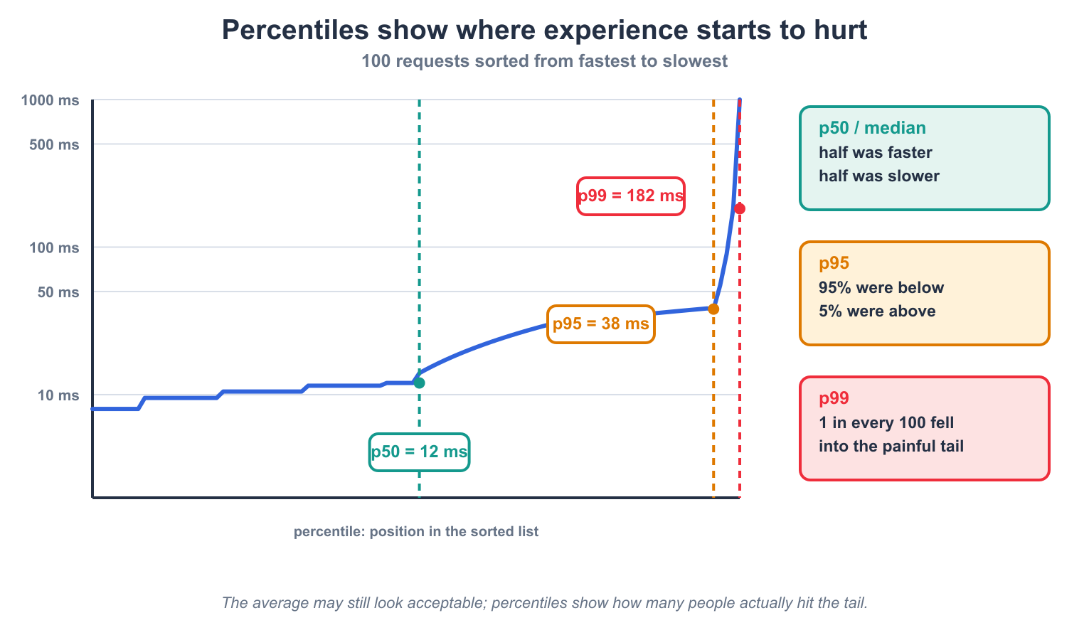
Percentiles are positions in a sorted latency list. The p50 describes the body of the distribution; p95 and p99 show where the tail starts to hurt.

A small example makes this clear. Imagine these ten latencies, already sorted:

10 ms, 11 ms, 11 ms, 12 ms, 12 ms, 13 ms, 14 ms, 15 ms, 18 ms, 500 ms

The average is 60.6 ms. It seems to say “the service is in the tens of milliseconds”. But nobody had exactly that experience. Nine calls were between 10 and 18 ms; one call took 500 ms. The average mixed two different realities and invented a number that represents neither. Worse, it softened exactly the event that defines the perception of whoever got the worst route. Percentiles make this mixture explicit: the body is fast, the tail is bad.

If you want to calculate percentiles in code, the conceptual version is this:

import math

def percentile(values, p):
    sorted_values = sorted(values)
    index = math.ceil((p / 100) * len(sorted_values)) - 1
    index = max(0, min(index, len(sorted_values) - 1))
    return sorted_values[index]

latencies = [10, 11, 11, 12, 12, 13, 14, 15, 18, 500]

print(percentile(latencies, 50))  # 12
print(percentile(latencies, 90))  # 18
print(percentile(latencies, 99))  # 500

This example is not a perfect implementation for every statistical percentile method, different libraries interpolate in different ways, but it captures the main idea: sort the latencies and look at the position you promised to protect. For resilience, that question matters more than the average, because the user does not feel the average. They feel their own request.

At scale, 1% is not small. In a system with 5,000 requests per second, p99 represents 50 requests per second above that threshold. That is 3,000 per minute. More than 4 million per day. This is why the tail of the distribution is not a statistical detail; it is a continuous slice of users crossing the worst version of your system.

I like Marc Brooker’s perspective: we can make the mistake of looking at p99.9 and concluding that it does not matter, after all 999 out of 1,000 calls see a latency lower than that. The problem, as he points out, is that modern architectures have many components, so a single user interaction can translate into many service calls.

It is this multiplication in distributed systems that turns a rare event into a common one.

Tail latency: when the tail dominates the system

Returning to this point and going deeper, in 2013 Jeffrey Dean and Luiz André Barroso published The Tail at Scale in Communications of the ACM. The paper introduces a central concept for this topic: just as distributed systems are designed to be fault-tolerant, they also need to be designed to be tail-tolerant, building a predictably responsive whole from parts that are individually less predictable. The parallel is direct: fault-tolerant computing creates a reliable whole from less reliable parts; tail tolerance creates a responsive whole from less responsive parts.

Because of the nature of distributed systems and their many parts, there is a lot of variability. It is worth understanding why this variability is inevitable: it is a consequence of shared systems. Contention for shared resources, background processes consuming CPU for a few milliseconds, maintenance activity such as compaction and garbage collection, queuing across multiple layers, and even hardware characteristics. One example from the paper: SSD garbage collection can increase read latency by a factor of 100 with only modest write activity happening in parallel.

Imagine a server that normally responds in 10 milliseconds, but whose p99 is 1 second, meaning 1 in every 100 responses is slow. If a user request touches only one of these servers, only 1 in every 100 requests becomes slow. In isolation, 1% looks small. But distributed systems rarely touch only one server. They fan out, firing dozens or hundreds of calls in parallel and waiting for all of them to return before assembling the final response, like a search request that queries 100 shards or a timeline that aggregates dozens of services. In that scenario, if you need to collect responses from 100 servers in parallel, then 63% of user requests will take more than one second.

That request or replica that becomes much slower than the others is called a straggler. Think of it as the delayed call in the group: it has not necessarily failed, it just fell behind. The problem is that in fan-out, the final response usually waits exactly for whoever fell behind.

One percent of slowness on each individual server became sixty-three percent of slow requests at the user level. If each call has a 99% chance of being fast, the chance that all 100 are fast is 0.99 multiplied by itself 100 times:

P(none of the 100 is slow) = (0.99)^100 ≈ 0.366
Therefore, P(at least one is slow) = 1 - 0.366 ≈ 0.634, or 63.4%.

The general formula is worth remembering:

P(at least one delayed request) = 1 - (1 - p)^N

p = probability of an individual call being slow · N = fan-out size. The tail does not add up: it composes. That is why it grows so fast.

The image below shows this curve for three levels of individual “bad luck”. What it shows is that the more your architecture spreads out, the more the tail stops being the exception and becomes the rule.

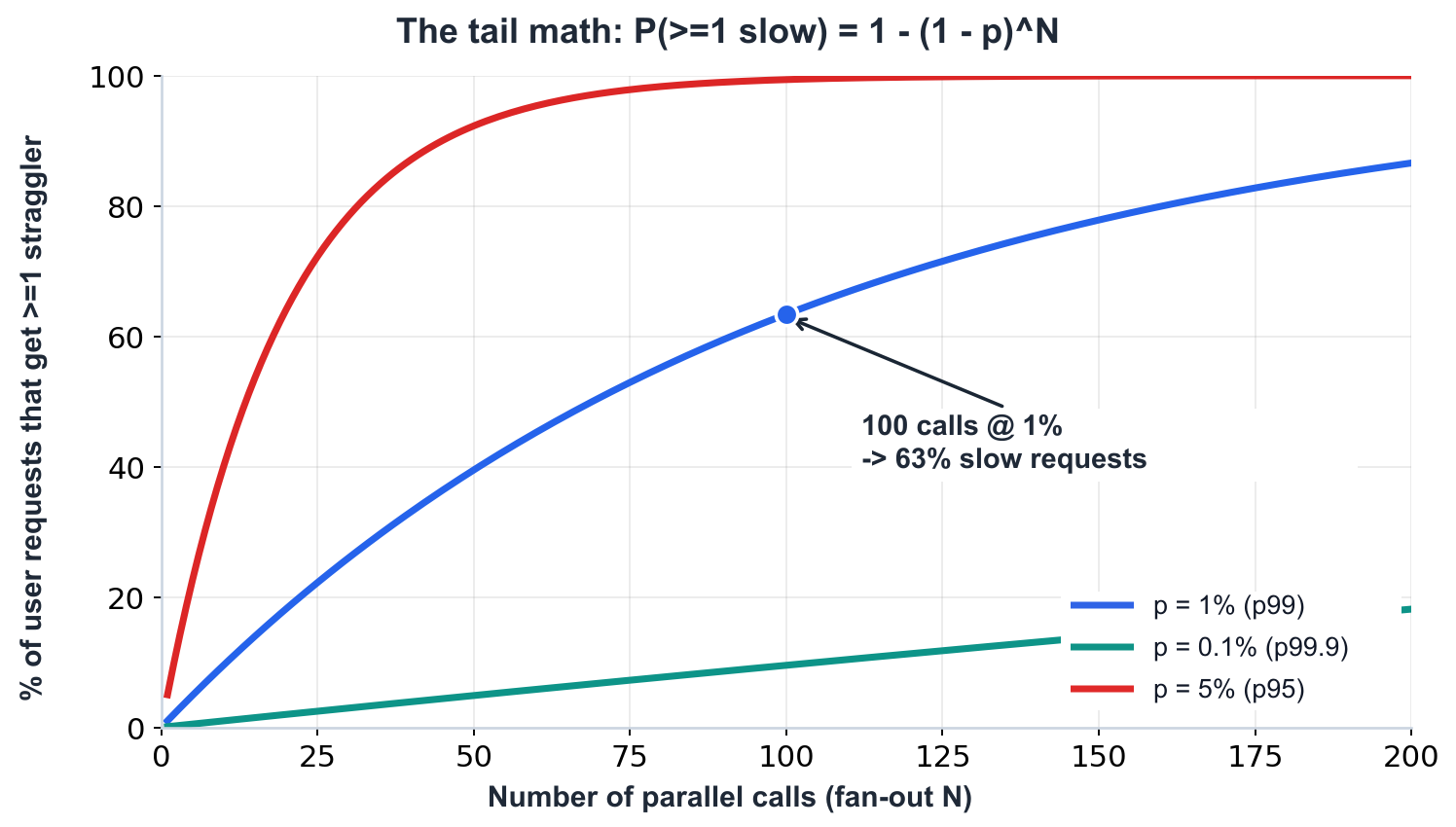
P(>=1 slow) = 1 - (1 - p)^N, for three levels of individual bad luck. With p = 1% (blue), 100 parallel calls make 63% of user requests hit a delayed call. Even with p = 0.1% (green), the tail reaches you; it only needs more fan-out. With p = 5% (red), a little more than 50 calls are enough to exceed 90%.

[[tail-latency-simulator]]

Notice the shape with p = 1%: you go from 1% impact in one call to almost 10% in ten calls, and to 63% in one hundred. Even with a probability ten times lower (p = 0.1%, the green line), the tail appears when fan-out grows. The paper shows this extreme even more dramatically: even with only 1 in 10,000 requests exceeding 1 second at the server level, a service with 2,000 servers will see almost 1 in 5 user requests exceed 1 second.

Besides parallel fan-out, there is serial chaining. When one service calls another, which calls another, the final latency is the sum of latencies across the chain. Imagine two worlds with the same average: one with a bimodal tail (99% of calls around 10 ms, 1% around 100 ms) and another with no tail at all. The simple existence of that rare 1% tail makes the variance of the distribution to which the chain converges, by the central limit theorem, 25 times larger than it would be in the world without a tail. Whether in parallel or in series, the tail appears in the composition.

The practical implication is that optimizing an isolated service may not move the system p99 if the problem is in the fan-out composition. Instead of asking “which service is slow?”, we should ask “how does the system avoid depending on the slowest participant in that composition?”. That is the question hedging answers.

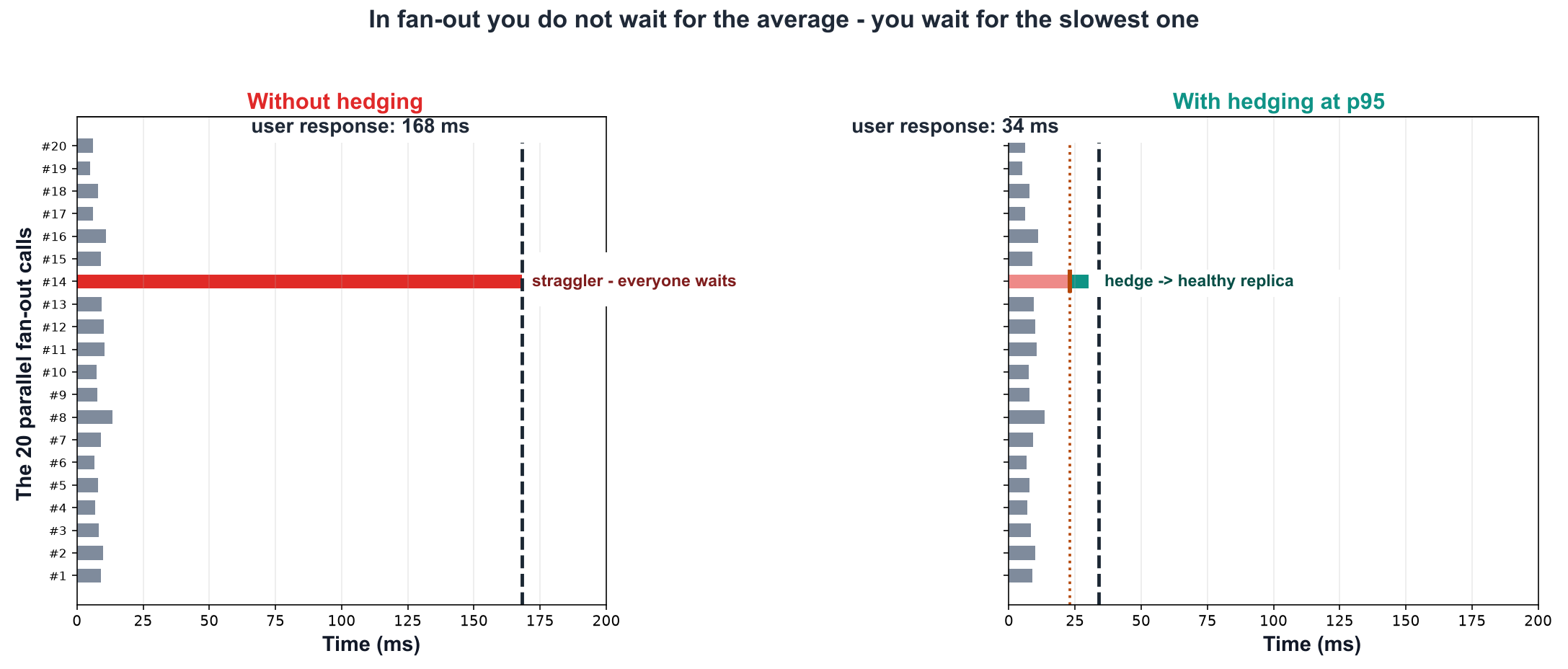
The same request, with a single unlucky call among 20 parallel calls. Without hedging, the user response is dictated by the slowest one (168 ms). With a hedge fired at p95, the straggler is bypassed and the response drops to 34 ms, without changing any of the other 19 calls. You do not wait for the average; you wait for the worst case.

Why p95 is a good starting point

In The Tail at Scale, Dean and Barroso measured a real Google service with a fan-out tree: a root talks to intermediate servers, which in turn talk to a large number of leaf servers, the leaves that actually do the work. They measured latency at three moments: when any leaf finishes, when 95% of leaves finish, and when 100% finish.

The p99 of an individual request, measured at the root, is only 10 ms. But the p99 for all requests in that fan-out to finish is 140 ms. And the p99 for 95% to finish is 70 ms. Do the math: the difference between waiting for 95% (70 ms) and waiting for 100% (140 ms) is 70 ms, exactly half of the total. Waiting for the slowest 5% of requests is responsible for half of the total p99 latency.

In practical terms, half of tail latency comes from the last 5% of responses. If there is a controlled way not to wait for those 5%, for example to work around the server that had a GC pause or a contention spike at that moment, the application reduces an important part of its exposure to the tail. This is the problem the hedging pattern attacks.

The importance of independence between paths

Return to the list of variability causes and assess how many are independent between replicas. Contention for a shared resource? No: it is the same switch, the same volume, the same database node behind both replicas. Maintenance activity triggered by the same scheduler? Correlated. A hot partition? That is the opposite of independent: both replicas serve the same partition, so hedging sends the copy straight to the same bottleneck.

The math makes this precise. For two events with the same probability p and correlation coefficient rho:

P(A slow AND B slow) = p^2 + rho * p * (1 - p)

With rho = 0, you recover the p^2 from the slide. But a little correlation is enough for the linear term to dominate, because p^2 is tiny and p * (1 - p) is not. With p = 1%:

`rho`	P(both slow)	equivalent to	P(B slow \| A slow)
0 (independent)	0.010%	1 in 10,000	1%
0.1	0.109%	1 in ~917	11%
0.3	0.307%	1 in ~326	31%
1.0 (identical)	1.0%	1 in 100	100%

Read the last column: with correlation of only 0.3, knowing that A is slow means there is a 31% chance that B is also slow. The probability that looked quadratic starts behaving almost like a linear risk again. That is why we talk so much about independence when the subject is resilience, replicas in different AZs, different hosts, different network paths: it is literally the attempt to push rho close to zero. And that is why hedging against a hot partition does not help. There, rho is 1, and the second attempt only adds load to the bottleneck.

Tied requests: cancellation before duplicated work

The hedging pattern has a small window of vulnerability that is worth understanding, because it motivates a more sophisticated variation. Between the moment you fire the backup and the moment the first response arrives, both servers may be executing the same thing at the same time. You limit that waste by waiting until the p95 before firing, but this, in turn, restricts the benefit to a small fraction of requests, only the ones that crossed the p95. It is a balance: the longer you wait, the less waste and the less benefit; the less you wait, the more of both.

Still in The Tail at Scale, the authors propose a more aggressive alternative: tied requests. An important observation: tied requests are not a client pattern. You do not implement this alone, from your side. They require three things outside the reach of someone who is only the client of a request: modifying servers so they understand a backup request marker and trigger request cancellation; a server-to-server cancellation channel between replicas; and a network between them that is faster than the work to be saved. That is why this technique lives inside storage systems and distributed databases, built by the server owners, not in a client library. This section serves as a reference for what is possible when you control both sides.

In this scenario, you send the request to two servers almost at the same time, but each copy carries the identity of the other server: they are “tied” to each other. The trick is the cancellation moment. When one of the servers starts executing the request, not when it finishes, but when it starts processing, typically by taking it out of its local queue, it immediately sends a cancellation message to its pair. The paper adds a practical detail: the client introduces a small delay, around twice the average network message latency, between the two copies to avoid sending both when both queues are empty.

Why does canceling when work starts, rather than when work finishes, make such a difference? Because most tail latency comes from queue time, not processing time. A server is usually slow because the request waited behind others in the queue, not because the operation itself is slow. By tying the two copies and canceling at the moment one leaves the queue and starts running, you ensure that the work is effectively done only by whoever got the request first; the two servers almost never process it in duplicate.

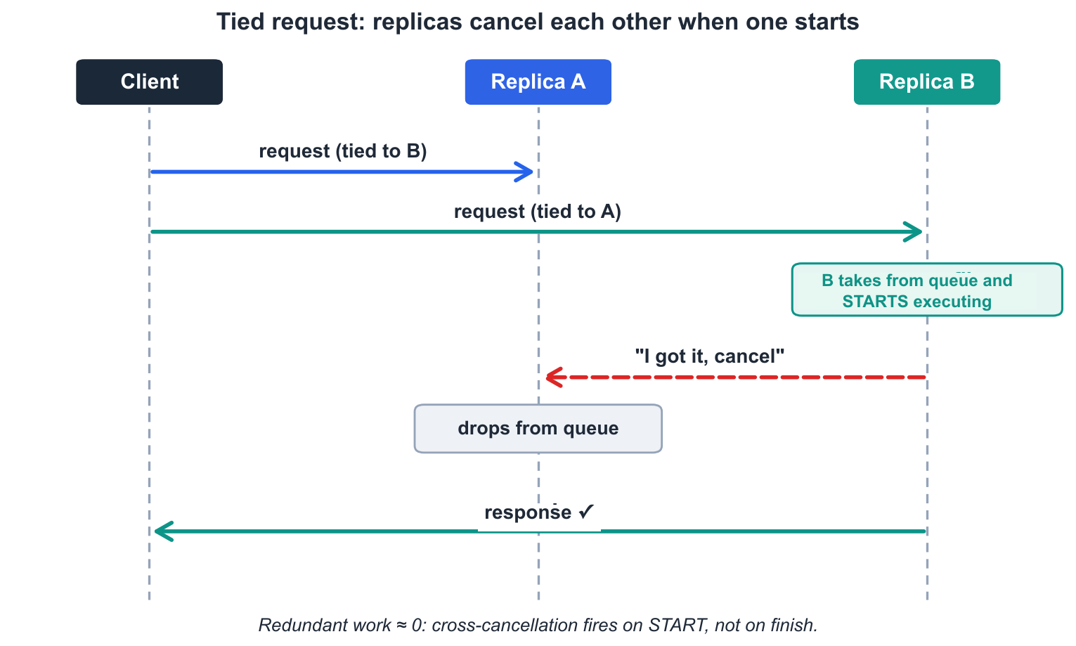
The empirical result is what supports the argument. In the scenarios tested in the paper, tied requests overhead in disk utilization stayed below 1%, indicating that the cancellation strategy effectively eliminates redundant reads. The most operationally relevant point is that the latency profile of a busy cluster, running a heavy sorting job in parallel and using tied requests, became almost identical to the latency profile of an idle cluster without tied requests. The practical reading is that the system can absorb more work in the same fleet, with better utilization and lower cost, without exposing clients to tail latency. We also cannot forget that we are discussing request journeys that may cross multiple layers of distributed services, which is why this approach pays off in the numbers.

Reducing tail exposure in an authorization flow with the hedging pattern on Amazon DynamoDB

Theory and papers are important, but the architectural value of hedging appears better when we look at a critical flow. In an AWS post, a payment processor running a credit card authorization platform on DynamoDB, designed to handle hundreds of millions of transactions per day and peaks of 5,000 transactions per second, found a typical problem in distributed systems at scale: the platform met the SLA up to the 95th percentile, but showed elevated latencies at p99 and p99.9 during performance tests.

The point is that an authorization flow became less exposed to the worst transient behavior of a dependency. At 5,000 TPS, p99 represents about 50 transactions per second above that threshold. In a payment system, that means dozens of authorizations per second crossing the worst version of that path at that moment. Reducing this exposure is a resilience gain: fewer transactions depend on the slowest path of the dependency.

They used the hedging pattern when the initial request to DynamoDB exceeded a time threshold: the system automatically fired a second request and used whichever responded first. The reported result was a 30% reduction in p99 latency. That number matters because it measures tail reduction, but the architectural reading matters more: fewer transactions were stuck in the worst available path at that moment.

It is also important to understand the type of independence and risk this case assumes. Hedging in the SDK against DynamoDB does not explicitly choose two independent replicas. It is the same endpoint, the same key and the same logical partition. The post itself makes clear that, in this design, SDK hedging mainly addresses network latency, a new connection, another path and another queue position, not storage node contention. The gain comes from reducing exposure to jitter and transient path variation, not from solving structural partition saturation.

What I found most interesting is the analysis of the delta value, the waiting time before firing the hedge. Different firing points were tested using GetItem, measuring both p99 improvement and duplicated request rate. The result shows why hedging needs to be calibrated as a resilience mechanism, not as aggressive duplication:

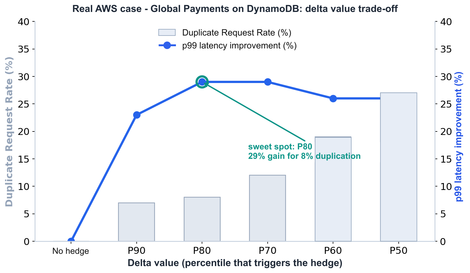
On the blue axis, p99 latency improvement; in the bars, the duplicated request rate. P80 is the balance point: 29% improvement for 8% duplication. From there, the gain plateaus and regresses, 26% at P60 and P50, while duplication jumps to 27%.

P90 brought 23% improvement with 7% duplicates. P80 brought 29% with 8%. After that, firing the hedge earlier stopped buying proportional resilience: at P50, the gain dropped to 26% while duplication rose to 27%. In DynamoDB, which charges per call, this duplication is direct cost. At the scale of the case itself, 5,000 TPS with 8% duplication means about 400 extra reads per second; with 27%, it means 1,350 extra reads per second.

Hedging increased the resilience of the flow by reducing transaction exposure to the tail of a dependency, within a measured duplication limit. The pattern should not be evaluated only by “how much it reduced p99”, but by how much it reduced the propagation of internal variation without turning that protection into uncontrolled load.

There is a catch: redundant work amplifies incidents

Hedging is, at its core, early speculative retry: you fire copies of requests expecting one of them to be faster than a designed target. Redundant requests without a brake are not resilience; they are a load amplification mechanism.

To understand the risk, it is worth comparing it with retry. The problem is what happens when retry meets a system already under stress, consumes even more resources and produces a retry storm. This is why the recommendation is to use adaptive retry with a token bucket, following current practices. Retry exists to increase the chance of success, but under overload it can consume the resources the service would need to recover.

This effect has a name: metastable failure. A system enters a metastable state when three things align: it is in a vulnerable state, close to its capacity limit; a trigger causes temporary overload; and that overload triggers a sustaining effect, typically work amplification coming from an optimization of the common path, such as retries or redundant requests. The feature that makes metastable failure so dangerous is this: the system does not recover on its own even after the original trigger disappears. The amplification cycle feeds itself and keeps the system degraded. The diagram below shows the anatomy of that loop.

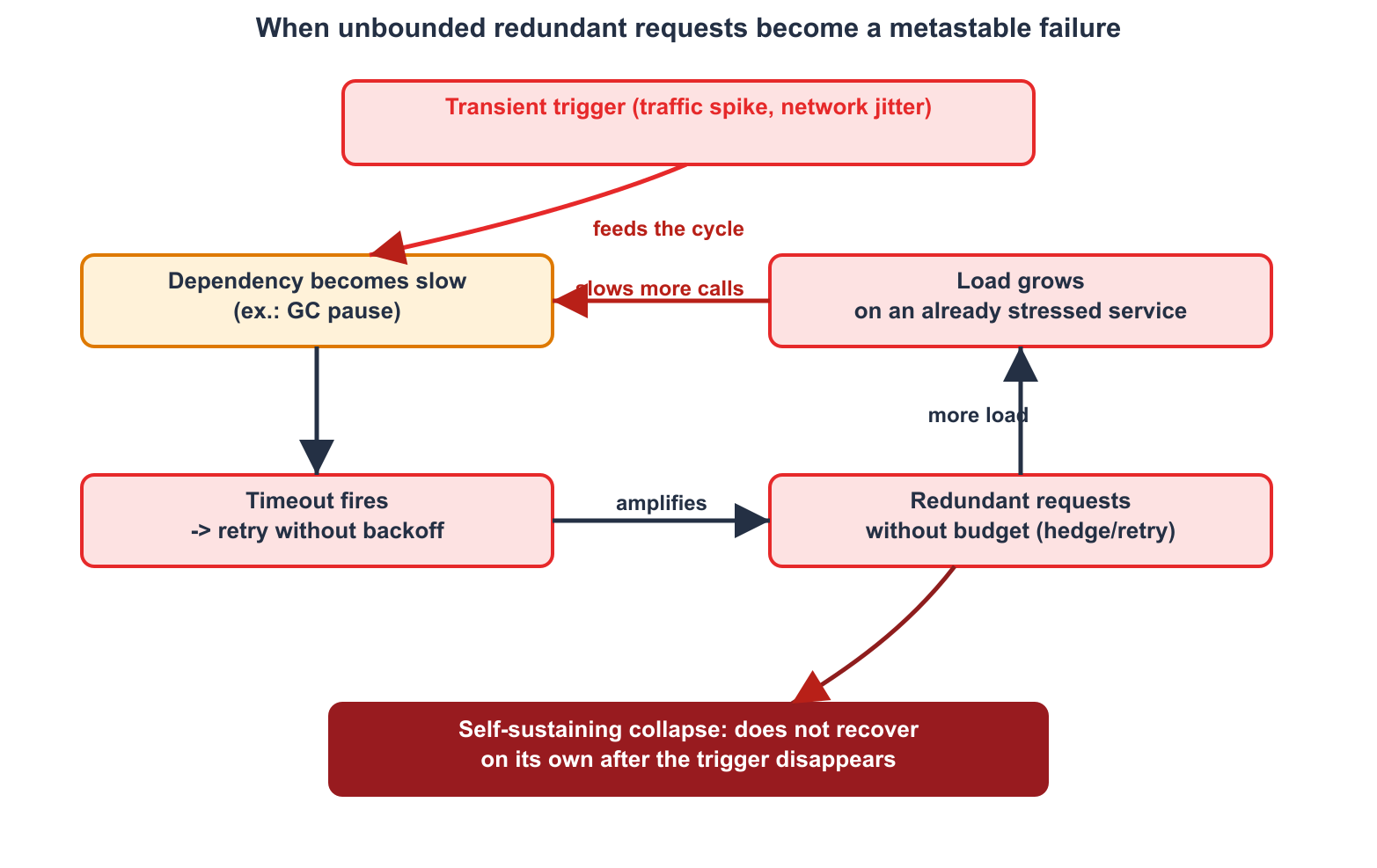
A typical metastable loop: the mechanism that should mask the failure starts amplifying work exactly when the service is already under stress.

In the post Erasure coding VS tail latency, this is connected directly to hedging. The argument is that the original paper’s claim that hedging does not add significant load tends to collapse exactly in failure cases, when we apply the lens of metastable failures. The described scenario is plausible: the p95 rule normally limits hedges to around 5%, but what if there is a correlated latency increase across the entire system, caused by traffic, an infrastructure failure or an empty cache, that raises all latencies up to the expected p95? At that moment, until the p95 expectation is updated, traffic can double and also receive cancellation traffic on top. In other words, hedging calibrated to fire on the slowest 5% fires for 100% of requests exactly during an incident, the worst possible time to double load.

Why 5% extra load does not cost 5% latency

A common question is: if I make another request for the slowest 5%, will that not cost me the same amount in latency? There is a common error in this question. When we say hedging costs only 5% extra requests, the cost is being measured in the wrong unit. The real impact appears in latency, and the relationship between load and latency depends on where the system is on the utilization curve.

The intuition comes from queueing theory. Take the M/M/1 model as an example, which says that the faster work arrives compared with the capacity to execute it, the longer each job waits. Response time scales with 1 / (1 - rho), where rho is resource utilization. While rho is low, adding load barely hurts. Close to saturation, the curve becomes a wall:

Utilization `rho`	Waiting factor `1/(1-rho)`	After +5% load
0.50	2.0x	2.1x
0.80	5.0x	6.3x (+25%)
0.90	10x	18x (+82%)
0.95	20x	400x (+1900%)

Read the rho = 0.90 row: 5% extra load does not cost 5% latency; it costs 82%. That is why hedging is dangerous under stress. In normal operation, with low rho, it can be almost free. But if hedging fires exactly when things are slow, and slow often means high rho, the application injects that 5% at the point of the curve where 5% load becomes a large fraction of latency. That makes more requests cross the p95 and fires more hedges. It is the metastable loop from the diagram, now with the explicit conversion: extra load turns into latency at a rate that grows near saturation.

The recommendation to control this risk is to always combine the technique with a token bucket approach that limits additional requests to what was expected. We can use 5% as an example, calibrated by the percentile where the hedge fires, and observe that the same token bucket used for adaptive retries works well here. We will return to that later in the post.

Token bucket as an amplification limit

The token bucket is the explicit limit that prevents hedging from growing together with the degradation. In normal operation, it allows a small number of speculative requests. During a correlated latency incident, when almost every request crosses the firing threshold, it prevents the system from doubling load. An emergency mechanism without a ceiling is not protection; it is a work multiplier.

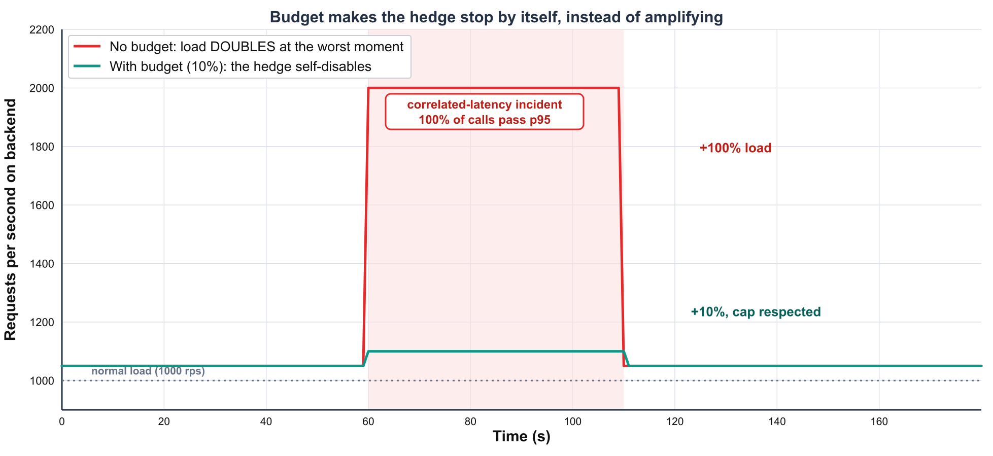
During a correlated latency incident, the red band, 100% of requests cross the p95 and become hedge candidates. Without a budget, backend load doubles, exactly at the worst moment. With a 10% token bucket, the bucket empties in the first moments and hedging stays within the ceiling you authorized: +10%, not +100%.

Because hedging is retry fired earlier, even before the first request fails. It inherits all of these amplification risks, with an important aggravating factor: it fires exactly in latency tails, meaning exactly during stress. Without idempotency, without cancellation and without a quota brake, your hedge is not protection. It is an incident waiting to happen. This is why the Well-Architected guidance is emphatic about configuring a maximum number of attempts or elapsed time, specifically to avoid backlogs that produce metastable failures.

Principles for using the hedging pattern safely

The following three principles define the boundary between reducing exposure to the tail and creating an incident amplification mechanism.

Idempotency is mandatory, not optional

Hedging duplicates requests by definition. If the operation has a side effect, a write, a charge, a state mutation, it will execute twice. Charging the customer twice in this case is not a bug; it is the direct and predictable consequence of using the hedging pattern on a non-idempotent operation. The AWS case illustrates this in practice: they apply hedging to reads of balance and history, which are naturally idempotent, but process the subsequent balance updates without hedging to preserve transactional integrity.

Reads are the simple case. For writes, use an idempotency token, and most implementations get wrong a detail that hedging guarantees will appear: the race between the two copies. The key must come from the business intent, generated once by the caller, a UUID per payment, not per attempt. If each hedged request generates its own key, there is no deduplication; there are two distinct operations with different names. And because hedging makes both arrive almost together, the backend needs to deduplicate with a conditional write, an atomic “insert only if this key does not exist yet”, not with “read then write”, which is exactly the window where both copies pass the test at the same time and both write.

Cancel the loser, always

When one response wins, whether primary or hedge, all requests still in flight must be canceled. But keep this in mind: canceling on the client does not stop work on the server. task.cancel(), ctx.cancel(), closing the socket, all of this frees your resources: the connection, thread, pool slot, buffer. That is a real gain, and it is the reason the rule exists. What does not happen is the server abandoning the work. It only does that if it was programmed to do so, if the handler propagates the cancellation context and checks whether the client is still there. Most frameworks do not do that by default. So cancellation protects the client from leaking resources, not the backend from duplicated load. What protects the backend is the extra load budget, not cancellation.

With that caveat, cancel anyway. If you do not cancel the loser, each hedge leaves an orphan request consuming a connection, thread or pool slot. Under load, this accumulation can exhaust client resources and turn an attempt to reduce tail latency into a local exhaustion failure.

This point matters because consuming a connection hides a counterintuitive mechanism: hedging can create the straggler it intended to bypass. Almost every HTTP client has a connection cap per host. When the pool for that host is full, the next call does not fail; it waits in the client queue. This wait appears in the measurement as call latency, indistinguishable from a slow server. The loop becomes: hedges fill the pool, new calls queue in the client, measured latency rises, more calls cross the p95, more hedges fire. The system starts generating stragglers inside its own process. This is why the absolute cap on in-flight requests and the pool sizing are not details; they are part of the resilience control.

There is a legitimate design decision here. In the AWS case, they chose to keep both requests active and monitor them simultaneously, letting the two compete, instead of canceling the first when firing the second. This is acceptable when the cost of letting both finish is low, such as a small and cheap read. But the decision must be deliberate: either you actively cancel to free your resources, or you guarantee that letting both run is cheap enough. What you cannot do is ignore the question.

Budget for extra load

This is the rule that controls amplification. You need two simultaneous limits. First, an absolute cap, a maximum number of in-flight requests per operation. In practice, hedging beyond 2 or 3 rarely pays off; gRPC, for example, which supports native hedging in service config, limits the number of attempts to a maximum of 5. Second, and more important, a proportional cap: a token bucket that limits hedging rate to a fraction of total traffic, 5% for example as a reference. In the code below, I use 10% as an example. With a 10% budget, you add at most 10% extra requests, never double, even if suddenly 100% of requests become slow.

During a correlated latency incident, all requests may become slow at the same time and all may become hedge candidates. Without budget, the application doubles load. With the token bucket, hedging saturates at the authorized rate. It does not go to zero; it is limited to, for example, +10%. The guarantee is not “zero extra load during the incident”; it is “extra load limited by a constant chosen before the incident”. The difference between +10% and +100% load on a degraded backend may be the difference between degradation and collapse.

There is an important refinement, used by production implementations such as gRPC: instead of calibrating the bucket by an “estimated RPS”, count real traffic. Each successful request deposits a fraction of a token; each hedge withdraws one full token. This way, the ceiling of “1 hedge every N requests” maintains itself, whether the service is at 5 rps or 50,000 rps, without manually estimating volume. The bucket also naturally shrinks when successes stop arriving. The code below uses this version. It is the same concept of adaptive retry used in the latest AWS SDK versions.

Budget in fan-out calls

Before leaving this section, we need to close a point left open by the tail math. The problem was built on fan-out, 100 parallel calls, 63% slow requests, but the rules were described as if there were only one call. It is not the same thing, and the difference changes sizing.

Fan-out is where hedging is often most valuable, because the user is not waiting for one response; they are waiting for the last of many. If half of p99 comes from waiting for the slowest 5%, hedging exactly those stragglers is a direct form of tail tolerance. But the cost also composes: if you hedge the slowest 5% of each of the 100 leaves, the expected number of hedges per user request is not “5% of one call”; it is 5% of 100, meaning five hedges in flight for that request. The budget, described earlier per operation, needs to be reasoned about across the whole fan-out: 5% extra load measured at the leaf becomes a much larger amount of parallel work at the user level. Define the budget and absolute cap with fan-out width in mind, not an isolated call. Otherwise, the budgeted “+5%” can become an unsized burst of work.

An implementation example

The goal of the code below is to show which controls must exist in a safe implementation. The implementation uses Python with asyncio, because the asynchronous nature makes the “fire two attempts and use the first valid response” logic explicit and readable.

Before the safe version, it is worth looking at the naive implementation, because it looks reasonable at first:

# Hedge without control/limit: fires both ALWAYS, without a brake, deadline or cancellation.
async def get(urls):
    tasks = [asyncio.create_task(client.get(u)) for u in urls]  # fires ALL
    done, _ = await asyncio.wait(tasks, return_when=asyncio.FIRST_COMPLETED)
    return done.pop().result()
    # three problems: (1) doubles load on 100% of traffic, not on the slowest 5%;
    # (2) nobody cancels the loser -> leaks connections;
    # (3) a fast failure becomes the "winner" and ends the good request behind it.

This snippet can reduce the tail in a local test and still amplify load in production. The safe version must include the three principles: idempotency, cancellation and budget.

First, the limit. The central component is the token bucket proportional to real traffic discussed in the budget section, with the same shape as gRPC’s hedging throttle, no estimated RPS: each success deposits tokens and each hedge withdraws one.

import asyncio
import time

class HedgeBudget:
    """
    Token bucket based on the real TRAFFIC RATIO, the budget brake.

    Each successful logical request deposits 'ratio' tokens; each hedge fired
    withdraws 1. With budget_percent=10, at equilibrium hedges do not exceed
    1 in every 10 requests, whether the service runs at 5 rps or 50,000 rps.

    Second-order effect, exactly the point of the budget: during an incident,
    successes stop arriving, the bucket stops filling, and hedges saturate at
    the ceiling you authorized, for example +10%, instead of doubling load.
    Single-threaded under asyncio: no lock needed.
    """
    def __init__(self, budget_percent: float = 10.0, burst: int = 10):
        self.ratio = budget_percent / 100.0
        self.capacity = float(burst)     # maximum burst of "stored" hedges
        self.tokens = float(burst)

    def on_success(self) -> None:
        """Every successful logical request credits the bucket."""
        self.tokens = min(self.capacity, self.tokens + self.ratio)

    def try_take(self) -> bool:
        """Tries to spend 1 token to hedge. Empty bucket -> DO NOT fire."""
        if self.tokens >= 1.0:
            self.tokens -= 1.0
            return True
        return False   # graceful degradation, without amplification

Now the hedge itself. The difference from the naive example is in three points: there is a deadline inherited by the hedge, a failure fires the hedge immediately instead of ending the operation, and the finally awaits cancellations before returning.

class AllReplicasFailed(Exception):
    pass

async def hedged_get(client, urls: list[str], hedge_delay: float,
                     budget: HedgeBudget, deadline: float,
                     max_in_flight: int = 2):
    """
    Executes a request with hedging.

    PRECONDITION (idempotency): 'urls' must point to an
    idempotent operation (a GET, or a backend with dedup). Never pass
    a non-idempotent write through here.

    hedge_delay: the "firing delay". Must be >= observed p95 of the target, so
    that the hedge only fires on the slowest ~5%. Calibrate with real data.
    deadline: TOTAL time (seconds) for the entire operation, inherited from
    the caller. It is NOT optional: without it, if no one responds, the loop
    spins forever, the backlog factory that Well-Architected
    tells you to avoid. The hedge inherits the time that was LEFT, never a new clock.

    Note: whoever operates this hedged_get credits the budget by calling
    budget.on_success() on each successful logical request (it is the credit
    that sustains the proportional cap). Omitted here to focus on the loop.
    """
    loop = asyncio.get_running_loop()
    end = loop.time() + deadline
    tasks = [asyncio.create_task(client.get(urls[0]))]
    next_url = 1
    last_error: BaseException | None = None
    try:
        while True:
            remaining = end - loop.time()
            if remaining <= 0:
                raise TimeoutError("call deadline exceeded") from last_error
            # the hedge can NEVER exceed the caller's deadline
            done, pend = await asyncio.wait(
                tasks, timeout=min(hedge_delay, remaining),
                return_when=asyncio.FIRST_COMPLETED,
            )
            had_failure = False
            for t in done:
                error = t.exception()
                if error is None:
                    return t.result()          # legitimate winner: 1st GOOD response
                last_error = error              # loser with error: does NOT propagate yet
                had_failure = True
            tasks = list(pend)                  # 'pend' already excludes the completed ones

            # Hedges if the primary became a straggler (timeout) OR if it FAILED.
            # on failure, hedge NOW, a failure is not waited on; it is worked around.
            can = next_url < min(max_in_flight, len(urls))
            if can and (had_failure or budget.try_take()):
                tasks.append(asyncio.create_task(client.get(urls[next_url])))
                next_url += 1
            elif not tasks:
                # nothing in flight and cannot hedge -> honest failure, no spinning
                raise AllReplicasFailed(str(last_error))
    finally:
        # Cancel and AWAIT teardown, so the connection returns to the pool
        # before we return. Canceling without waiting leaks the connection and pollutes logs.
        for t in tasks:
            if not t.done():
                t.cancel()
        if tasks:
            await asyncio.gather(*tasks, return_exceptions=True)

Four points separate this version from the anti-pattern at the start of the section. First, the hedge fires one at a time and only after re-evaluating caps, never in a burst. Second, a fast failure from the primary fires the hedge immediately, without waiting for the delay and without ending the request. Third, there is a global deadline: if nobody responds, the operation fails in a bounded time instead of spinning indefinitely. Fourth, the finally not only cancels but waits for cancellation to propagate, returning the connection to the pool. The implementation was exercised in the cases of fast primary, hedge winner, fast failure, all replicas failing, total timeout and a single URL.

It is important to consider that, depending on the use case and service type, per-operation delay may matter, as in the AWS post involving DynamoDB. Each operation type has its own latency profile: a GetItem usually has lower latency than a Query returning 100 records or a Scan that reads whole pages, and this matters especially when the same application mixes operations. The source does not prescribe a delay per operation, but the practical conclusion is direct: if you use one global hedge_delay for operations with different profiles, you will hedge too early in some and too late in others. Measure each class and calibrate each one. AWS’s own tests, as in the Global Payments implementation, covered GetItem.

There is also the rollout question. The initial hedge_delay comes from a dashboard, and the real distribution in the code path may differ. If the estimate is wrong by a factor of three downward, the first deploy can hedge most of the traffic. That is why, before enabling hedging, run in shadow mode: the entire decision logic executes, timer, percentile estimate, cap, budget, but at the point where it would fire the hedge it only records a metric, “would have hedged now”, instead of sending the second request. This creates zero extra load and reveals the real firing rate. Only after that does it make sense to enable it for real, for a small fraction of traffic, with a kill switch by configuration, not by deploy.

Metrics to operate hedging in production

Hedging fails silently in both directions, and neither appears in a common latency dashboard. Calibrated too high, it costs money without reducing the tail. Calibrated too low, it amplifies. Before turning this on in production, instrument four metrics.

1. Hedge rate: (hedges fired / calls, by operation class). This is the cost metric, and you have a declared target for it: the 5% to 10% you budgeted. Alarm on deviation, not on the absolute value. If it jumps from 5% to 40% in minutes, either your p95 estimate became obsolete or you are at the beginning of a correlated latency event.

2. Hedge win rate: (hedges that won / hedges fired). This is the effectiveness metric, and it reveals wrong calibration. If you fire hedges and they almost never win, your delay is too short; you are paying extra work for nothing. If they almost always win, your delay is too long and you are leaving latency on the table. A healthy number is intermediate: the hedge should win often enough to justify the cost, without always winning.

3. Latency with and without hedge, both side by side: Measure effective latency, the one that won, and the latency the primary would have had alone, always. The difference is the real gain from the hedge, measured continuously instead of assumed. This is the metric that answers whether the hedge is still worth it, instead of depending on the assumption created on rollout day.

4. Latency of the hedge path, separate from the primary: This is the alarm the rate budget does not cover. If your hedge goes through a path that can be an order of magnitude slower, another AZ, another region, a colder cache, a hedge that wins but takes ten times longer holds a pool slot for ten times longer and fills the pool with successful hedges. The hedge rate stays within budget and you still saturate through concurrency. Only a separate hedge path latency metric catches this before the incident.

With these four metrics, hedging stops being an invisible optimization and becomes an operable mechanism. With only aggregate latency, the system does not show when the pattern is amplifying load exactly when that is most dangerous.

When not to use hedging

Here is the list of situations where hedging is not the answer. This section is as important as the previous ones, because the pattern only increases resilience when applied to the right type of degradation. Each item ends with what to use instead of hedging.

Non-idempotent operations without deduplication: If the operation has a side effect and you do not have an idempotency token or backend deduplication, hedging will execute it twice. This is a structural restriction. Do not use hedging on writes as an uncontrolled experiment. Instead, make the operation idempotent first, client-generated key plus conditional write, and only then consider hedging.

Single-instance backends: The hedge wins because it races the backup against a different replica that probably is not having the same bad luck. If both requests go to the same machine, a single-instance backend or a cache without replicas, you worked around nothing; you only added load to the machine that was already slow. Instead, invest in replicas and redundancy before any hedge. Without low rho, hedging has nothing to buy.

Resource-saturated backends: This is the most subtle and most important distinction. Hedging works when slowness comes from transient and localized factors, a GC pause, a contention spike, network jitter, a momentary hot partition. In these cases, the second replica often reaches a healthy machine. But if slowness comes from sustained resource exhaustion, maxed-out CPU, degraded database, real saturation, then adding a hedge only worsens saturation. You are sending more work to a system that already cannot handle what it has. In that scenario, the hedge is the beginning of a metastable failure. The question that separates the two cases is: is the slowness punctual bad luck or lack of capacity? Instead, use load shedding, adaptive concurrency limits and backpressure, tools that remove work under stress, not add it.

Services behind a shared rate limit: If the backend enforces a global quota, a third-party API or a token-per-minute limit, hedge requests consume that quota. You may trigger throttling that would not otherwise happen, and then the “fix” for the tail becomes the cause of errors. Instead, use client-side quota and request prioritization, so the shared budget is not spent on speculative work.

Very low traffic services: Adaptive hedging, which learns the p95 in real time, needs volume to distinguish a straggler from normal variance. In a service receiving less than one request per second, there is not enough data to calibrate, and you end up hedging noise. Instead, a well-measured fixed timeout plus retry with backoff and jitter, or adaptive retry, solves the sporadic case without requiring statistics you do not have.

When failures are rare or transient, retries work well; when they are caused by resource overload, they can make things worse, and the same applies, by extension, to hedges. Hedging is a specific tool for reducing exposure to transient variation. It is not a solution for lack of capacity.

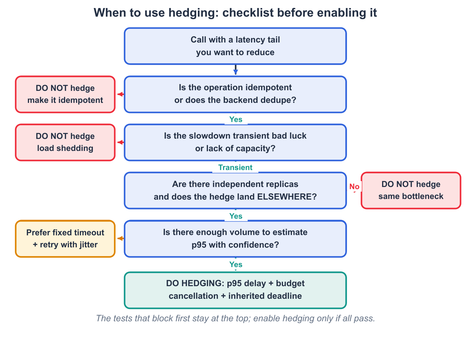
If you want a single artifact to take to your next design review, it is this, the tests in order, with the blockers first at the top:

Hedging and the constant work principle

Connecting this with the first article. In the constant work principle, the recommendation was to distrust emergency modes that only appear during a failure. Hedging also creates a second mode: in normal operation, one attempt; in the tail, an additional attempt.

The difference is what changes in the second mode. The dangerous fallback is the one that, under failure, starts doing different work, switches execution path, activates rarely exercised logic or changes the load profile into something that was not sized. The hedge does not do different work; it does more of the same work, against another compatible path or replica. The nature of the operation does not change, only the destination and the amount.

This defense only holds with a budget. Without a token bucket, hedging falls into the same pathology discussed in the first article: “1x normal, 2x under stress” can become “1x normal, 2x for all traffic at the same time during the incident”. In that case, the second mode amplifies the failure instead of containing it. What makes hedging acceptable is limiting the amplitude of the second mode to a small constant chosen before the degradation.

Alternatives to hedging

Hedging is one tool in a larger toolbox. Marc Brooker’s post is, in fact, an alternative and an argument for erasure coding as a more general alternative: instead of sending the same request twice, you split the data into M pieces recoverable from any k, fire all M, and respond as soon as the first k arrive. Brooker makes the trade-off explicit: this amplifies more requests than hedging, in his example 5x instead of 2x, but with lower bandwidth and storage cost, and it can improve even the median, not only the tail, because it is not modal. For caches and latency-sensitive storage systems, it is a relevant alternative.

Conclusion

The hedging pattern increases resilience when it reduces an application’s exposure to tail latency. It does not increase real capacity, it does not replace redundancy and it does not correct saturation. What it does is use existing redundancy in a speculative and limited way to prevent a transient and localized slowdown from defining the final response.

That distinction matters. If the slowness comes from a GC pause, network jitter, a local queue or a momentarily worse replica, hedging can mask the variation and keep the flow predictable. If the slowness comes from sustained saturation, a hot partition or lack of capacity, hedging adds work to the wrong place and can accelerate a metastable failure.

That is why, in my view, the pattern is only viable with three controls: idempotency, cancellation and budget. Idempotency prevents duplicated side effects. Cancellation avoids resource leaks in the client. Budget limits extra load when the degradation stops being localized and becomes correlated. Without these controls, hedging stops being resilience and becomes amplification.

Hedging increases resilience by accepting a small amount of redundant work to reduce exposure to the tail. These are different techniques, but they share the same operational principle: during a degradation, the system cannot amplify work without limit.

Before applying hedging to a critical service, answer objectively:

Is the operation idempotent or does it have atomic deduplication in the backend?

Can the hedge really follow an independent path, or will it hit the same bottleneck?

Is the slowness you want to mask transient and localized, or is it lack of capacity?

If 100% of requests cross the firing threshold, is there a budget that prevents doubling load?

The answer to the fourth question defines whether hedging increases the system’s resilience or only creates another failure mode.

References:

- cseweb.ucsd.edu/classes/sp18/cse124-a/post/schedule/p74-dean.pdf
- brooker.co.za/blog/2021/04/19/latency.html
- brooker.co.za/blog/2023/01/06/erasure.html
- https://aws.amazon.com/blogs/database/how-global-payments-inc-improved-their-tail-latency-using-request-hedging-with-amazon-dynamodb/
- https://docs.aws.amazon.com/wellarchitected/2024-06-27/framework/rel_mitigate_interaction_failure_limit_retries.html
- sigops.org/s/conferences/hotos/2021/papers/hotos21-s11-bronson.pdf
- grpc.io/docs/guides/request-hedging/
- https://docs.aws.amazon.com/sdkref/latest/guide/feature-retry-behavior.html